
본 포스팅은 kaggle:Intermediate Machine Learning을 수료하고 정리한 글입니다.
1. Introduction
Intro Machine Learning을 수료한 후 모델의 성능을 신속하게 향상시키기 위해 방법과 XGBoost에 대해서 학습할 것이다.
다음과 같은 학습내용으로 진행할 것이다.
- 결측치 처리
- 숫자형 변수, 카테고리형 변수에 대해서
- 파이프라인 설계
- 모델 검증(교차 검증)
- XGBoost
2. Missing Values
이 장에서는 결측치를 처리하는 세 가지 방법에 대해 알아볼 것이다.
2-1 개요
데이터는 여러 이유로 결측값을 가지게 된다. 예를 들어
- 데이터를 입력 중 실수로 값을 입력하지 않은 경우
- 값을 어떤 이유로든 관찰하지 못한 경우(예를 들어, 인구 조사에서 특정 가구가 구성원수를 기입하지 않은 경우)
- 해당 항목에 적절한 값이 없어서 입력하지 못한 경우(예를 들어, 약품의 냄새를 기록하는 칸에 특정 약품은 향이 없는 경우)
2-2 결측값 처리 방법
- 결측값이 있는 열 삭제(Drop Columns with Missing Values)
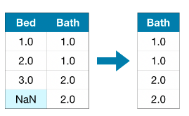
- 말 그대로 결측값이 있는 column은 삭제하는 것이다.
- 가장 간단한 방법이다. 제거되는 column의 대부분의 값이 결측값이 아니라면 많은 정보를 잃어버리는 결과를 초래하게 된다. 예를 들어 10,000개의 행을 가진 데이터셋에서 하나의 중요한 column이 1개의 결측치를 갖고 있다면 이러한 방법으로는 column 전체를 제거하게 될 것이다.
- 대치법(Imputation)
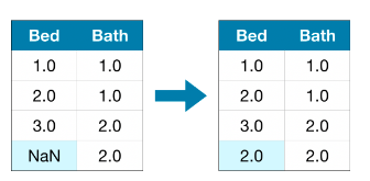
- 대치법은 결측값을 다른 값으로 대체하는 방법이다. 예를 들어 각 column별 결측치에는 각 column별 평균값으로 대체할 수 있다.
- 이렇게 채워진 값은 대부분의 경우 정확하지 않지만, 방법1보다는 더 정확한 모델을 만들 수 있다.
- 결측값 대체 후 데이터셋 확장(An Extension To Imputation)
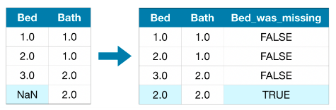
- 이 접근법은 2번과 마찬가지로 결측치에 값을 채워넣는다. 그 후 원래 데이터셋에 결측치가 있던 컬럼에 대하여 어떤 값이 채워진 값인지를 나타내는 column을 새로 만들어 낸다.
2-3 예제
예제에서는 Melbourne Housing dataset을 이용한다. 모델은 방의 개수, 부지의 크기 등을 이용하여 집의 가격을 예측하는 모델을 만들 것이다.
import pandas as pd
from sklearn.model_selection import train_test_split

# Load the data
data = pd.read_csv('../input/melbourne-housing-snapshot/melb_data.csv')

# Select target
y = data.Price

# To keep things simple, we'll use only numerical predictors
melb_predictors = data.drop(['Price'], axis=1)
X = melb_predictors.select_dtypes(exclude=['object'])

# Divide data into training and validation subsets
X_train, X_valid, y_train, y_valid = train_test_split(X, y, train_size=0.8, test_size=0.2,
random_state=0)3가지 방법의 성능을 측정하기 위한 함수인 score_dataset()를 정의한다. 이 함수는 random forest 모델로 계산된 평균절대오차(MAE : Mean Absolute error)를 반환해 준다.
(MAE : 실제 정답 값과 예측 값의 차이를 절댓값으로 변환한 뒤 합산하여 평균을 구한다. 값이 낮을수록 좋다.)
방법1 : 결측값이 있는 열 삭제
- 학습 및 훈련 데이터셋, 둘 다 사용하기 때문에 동일한 column을 두 데이터셋에서 제거해야 한다.
# Get names of columns with missing values
cols_with_missing = [col for col in X_train.columns
                     if X_train[col].isnull().any()]
# Drop columns in training and validation data
reduced_X_train = X_train.drop(cols_with_missing, axis=1)
reduced_X_valid = X_valid.drop(cols_with_missing, axis=1)
print("MAE from Approach 1 (Drop columns with missing values):")
print(score_dataset(reduced_X_train, reduced_X_valid, y_train, y_valid))MAE from Approach 1 (Drop columns with missing values):
183550.22137772635방법2 : 대치법(Imputation)
- SimpleImputer를 사용해서 결측값들을 각 column별 평균값으로 대체할 것이다.
- 간단한 방법이지만, 꽤 좋은 성능을 보인다.
from sklearn.impute import SimpleImputer
# Imputation
my_imputer = SimpleImputer()
imputed_X_train = pd.DataFrame(my_imputer.fit_transform(X_train))
imputed_X_valid = pd.DataFrame(my_imputer.transform(X_valid))
# Imputation removed column names; put them back
imputed_X_train.columns = X_train.columns
imputed_X_valid.columns = X_valid.columns
print("MAE from Approach 2 (Imputation):")
print(score_dataset(imputed_X_train, imputed_X_valid, y_train, y_valid))MAE from Approach 2 (Imputation):
178166.46269899711결과를 통해 방법2가 방법1보다 더 낮은 MAE를 보인 것을 확인할 수 있다.
방법3 : 결측값 대체 후 데이터셋 확장
- 결측값을 채워넣은 후, 채워진 값에는 True값을 넣는다.
# Make copy to avoid changing original data (when imputing)
X_train_plus = X_train.copy()
X_valid_plus = X_valid.copy()

# Make new columns indicating what will be imputed
for col in cols_with_missing:
    X_train_plus[col + '_was_missing'] = X_train_plus[col].isnull()
    X_valid_plus[col + '_was_missing'] = X_valid_plus[col].isnull()

# Imputation
my_imputer = SimpleImputer()
imputed_X_train_plus = pd.DataFrame(my_imputer.fit_transform(X_train_plus))
imputed_X_valid_plus = pd.DataFrame(my_imputer.transform(X_valid_plus))

# Imputation removed column names; put them back
imputed_X_train_plus.columns = X_train_plus.columns
imputed_X_valid_plus.columns = X_valid_plus.columns

print("MAE from Approach 3 (An Extension to Imputation):")
print(score_dataset(imputed_X_train_plus, imputed_X_valid_plus, y_train, y_valid))MAE from Approach 3 (An Extension to Imputation):
178927.503183954방법3은 방법2보다 MAE가 약간 높은 결과를 보인다.
왜 결측값을 대체하는 것이 column을 삭제하는 것보다 더 좋은 성능을 보여줄까?
: 학습데이터는 10864개의 행과 12개의 column을 갖고 있다. 3개의 column이 결측치를 갖고 있고, 각 column에서 결측값의 수는 전체 데이터 수의 절반 이하이다. 그러므로 column을 제거하면 많은 정보가 제거되기 때문에, imputation으로 결측값을 채워넣는 것은 column을 제거하는 것보다 더 좋은 성능을 보인다.
# Shape of training data (num_rows, num_columns)
print(X_train.shape)

# Number of missing values in each column of training data
missing_val_count_by_column = (X_train.isnull().sum())
print(missing_val_count_by_column[missing_val_count_by_column > 0])(10864, 12)
Car 49
BuildingArea 5156
YearBuilt 4307
dtype: int642-4 결론
일반적으로 결측값이 존재하는 column을 지우는 것보다 결측값을 어떠한 값(ex. 평균값)으로 채워넣는 것이 더 좋은 성능을 보인다.
3. Categorical Variables
이 장에서는 범주형 변수(Categorical Variable)가 무엇인지, 어떻게 다뤄야 할 지 대해서 학습할 것이다.
3-1 개요
범주형 변수는 가질 수 있는 값이 한정되어 있다. 예를 들어
- 얼마나 아침을 자주 먹는지에 대해 "먹지 않는다(Never)", "일주일에 1 ~ 3번(Rarely)", "일주일에 4 ~ 6번(Most day), "매일 먹는다(Every Day)라고 주어진 설문조사를 생각해보자. 이 경우 대답은 4가지 범주 중 하나를 선택해야 하기 때문에, Categorical Varible라고 할 수 있다.
- 만약 어떤 브랜드의 차를 소유하고 있나요? 라는 질문에는 아마 "KIA", "BMW", "Benz" 등으로 대답할 것이다. 이러한 경우에도 Categorical Varible라고 할 수 있다.
이러한 범주형 변수를 머신러닝 모델에 아무 전처리 없이 사용했다간 많은 어려움을 겪게 될 것이다!
3-2 범주형 변수 다루는 방법
- 범주형 변수 제거(Drop Categorical Variables)
- 단순히 범주형 변수는 제거하는 방법이다.
- 이 방법은 해당 변수에 중요한 정보가 없을 때만 효과가 있을 것이다.
- Ordinal Encoding
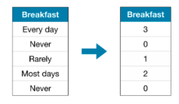
- 이 방법은 범주형 변수에 순서를 부여하는 것이다. (Never" (0) < "Rarely" (1) < "Most days" (2) < "Every day" (3))
- 위 예시에서는 각 범주의 순서가 있다고 판단되기에 가정이 적절하다고 볼 수 있다.
- 순서가 있는 범주형 변수를 순위변수(ordinal variable)라고 부른다.
- Decision tree, Random Forest 등 트리 기반의 모델에서 ordinal Encoding이 잘 작동한다.
- 원-핫 인코딩(One-Hot Encoding)
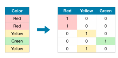
- 왼쪽 그림에 "Color"는 Red, Yellow, Green 3가지의 범주를 갖고 있는 변수형 변수이다. 각 범주마다 원-핫 인코딩된 컬럼을 가지고 있다. 만약 원래값이 "Red"일 경우 "Red" column에 1을 집어 넣는다.
- 2번 방법과 달리 원-핫 인코딩은 범주의 순서를 매기지 않는다. 이러한 순서가 없는 데이터를 명목형 변수(nominal variable) 이라 부른다.
- 원-핫 인코딩은 대체로 범주의 수가 15개 이하인 경우에 사용한다.
3-3 예제
이전 예제와 동일한 Melbourne Housing dataset를 이용한다.
import pandas as pd
from sklearn.model_selection import train_test_split

# Read the data
data = pd.read_csv('../input/melbourne-housing-snapshot/melb_data.csv')

# Separate target from predictors
y = data.Price
X = data.drop(['Price'], axis=1)

# Divide data into training and validation subsets
X_train_full, X_valid_full, y_train, y_valid = train_test_split(X, y, train_size=0.8, test_size=0.2,
                                                                random_state=0)

# Drop columns with missing values (simplest approach)
cols_with_missing = [col for col in X_train_full.columns if X_train_full[col].isnull().any()]
X_train_full.drop(cols_with_missing, axis=1, inplace=True)
X_valid_full.drop(cols_with_missing, axis=1, inplace=True)

# "Cardinality" means the number of unique values in a column
# Select categorical columns with relatively low cardinality (convenient but arbitrary)
low_cardinality_cols = [cname for cname in X_train_full.columns if X_train_full[cname].nunique() < 10 and
                        X_train_full[cname].dtype == "object"]

# Select numerical columns
numerical_cols = [cname for cname in X_train_full.columns if X_train_full[cname].dtype in ['int64', 'float64']]

# Keep selected columns only
my_cols = low_cardinality_cols + numerical_cols
X_train = X_train_full[my_cols].copy()
X_valid = X_valid_full[my_cols].copy()head() 메서드를 통해 학습데이터를 살펴보자
X_train.head()| Type | Method | Regionname | Rooms | Distance | Postcode | Bedroom2 | Bathroom | Landsize | Lattitude | Longtitude | Propertycount | |
|---|---|---|---|---|---|---|---|---|---|---|---|---|
| 12167 | u | S | Southern Metropolitan | 1 | 5.0 | 3182.0 | 1.0 | 1.0 | 0.0 | -37.85984 | 144.9867 | 13240.0 |
| 6524 | h | SA | Western Metropolitan | 2 | 8.0 | 3016.0 | 2.0 | 2.0 | 193.0 | -37.85800 | 144.9005 | 6380.0 |
| 8413 | h | S | Western Metropolitan | 3 | 12.6 | 3020.0 | 3.0 | 1.0 | 555.0 | -37.79880 | 144.8220 | 3755.0 |
| 2919 | u | SP | Northern Metropolitan | 3 | 13.0 | 3046.0 | 3.0 | 1.0 | 265.0 | -37.70830 | 144.9158 | 8870.0 |
| 6043 | h | S | Western Metropolitan | 3 | 13.3 | 3020.0 | 3.0 | 1.0 | 673.0 | -37.76230 | 144.8272 | 4217.0 |
데이터타입(dtype)을 통해 범주형 변수인지 아닌지를 확인할 수 있다. 주로 데이터타입이 object인 것은 범주형 변수임을 의미한다.(아닌 경우도 있음!)
# Get list of categorical variables
s = (X_train.dtypes == 'object')
object_cols = list(s[s].index)

print("Categorical variables:")
print(object_cols)Categorical variables:
['Type', 'Method', 'Regionname']3가지 방법의 성능을 측정하기 위한 함수인 score_dataset()를 정의한다. 이 함수는 random forest 모델로 계산된 평균절대오차(MAE : Mean Absolute error)를 반환해 준다.
from sklearn.ensemble import RandomForestRegressor
from sklearn.metrics import mean_absolute_error

# Function for comparing different approaches
def score_dataset(X_train, X_valid, y_train, y_valid):
    model = RandomForestRegressor(n_estimators=100, random_state=0)
    model.fit(X_train, y_train)
    preds = model.predict(X_valid)
return mean_absolute_error(y_valid, preds)방법1 : 범주형 변수 제거
select_dtypes() 함수를 이용해서 object 타입의 column을 찾아 삭제한다.
drop_X_train = X_train.select_dtypes(exclude=['object'])
drop_X_valid = X_valid.select_dtypes(exclude=['object'])

print("MAE from Approach 1 (Drop categorical variables):")
print(score_dataset(drop_X_train, drop_X_valid, y_train, y_valid))MAE from Approach 1 (Drop categorical variables):
175703.48185157913방법2 : Ordinal Encoding
scikit-learn의 OrdinalEncoder 클래스를 사용해서 값을 구할 수 있다.
from sklearn.preprocessing import OrdinalEncoder

# Make copy to avoid changing original data
label_X_train = X_train.copy()
label_X_valid = X_valid.copy()

# Apply ordinal encoder to each column with categorical data
ordinal_encoder = OrdinalEncoder()
label_X_train[object_cols] = ordinal_encoder.fit_transform(X_train[object_cols])
label_X_valid[object_cols] = ordinal_encoder.transform(X_valid[object_cols])

print("MAE from Approach 2 (Ordinal Encoding):")
print(score_dataset(label_X_train, label_X_valid, y_train, y_valid))MAE from Approach 2 (Ordinal Encoding):
165936.40548390493각각의 열에 무작위로 정수의 값을 할당했다. custom label를 만드는 것보다 간단하고 자주 사용된다. 하지만 만약 각 열에 많은 label를 만든다면 더 좋은 성능을 가진 모델을 만들 수 있다.
방법3 : One-Hot Encoding
scikit-learn의 OneHotEncoder 클래스를 사용해서 값을 구할 수 있다.
사용하기 전에 몇 가지 매개변수를 설정해줘야 한다.
- handle_unknown='ignore'을 설정하여 검증 데이터에서 학습데이터에서는 존재하지 않는 class을 만났을 때 발생하는 오류를 방지한다.
- sparse=False는 encode된 column이 sparse matrix 대신에 numpy array 형태로 리턴 되도록 설정해준다.
- encoder를 사용하기 위해 오직 원-핫 인코딩되길 원하는 범주형 변수만 넘겨줘야 한다.
from sklearn.preprocessing import OneHotEncoder
# Apply one-hot encoder to each column with categorical data
OH_encoder = OneHotEncoder(handle_unknown='ignore', sparse=False)
OH_cols_train = pd.DataFrame(OH_encoder.fit_transform(X_train[object_cols]))
OH_cols_valid = pd.DataFrame(OH_encoder.transform(X_valid[object_cols]))

# One-hot encoding removed index; put it back
OH_cols_train.index = X_train.index
OH_cols_valid.index = X_valid.index

# Remove categorical columns (will replace with one-hot encoding)
num_X_train = X_train.drop(object_cols, axis=1)
num_X_valid = X_valid.drop(object_cols, axis=1)

# Add one-hot encoded columns to numerical features
OH_X_train = pd.concat([num_X_train, OH_cols_train], axis=1)
OH_X_valid = pd.concat([num_X_valid, OH_cols_valid], axis=1)

print("MAE from Approach 3 (One-Hot Encoding):")
print(score_dataset(OH_X_train, OH_X_valid, y_train, y_valid))MAE from Approach 3 (One-Hot Encoding):
166089.4893009678어떤 방법이 가장 좋을까?
위 예제에서는 방법1(범주형 변수 제거)이 제일 안 좋은 성능을 보였다. 다른 두 방법같은 경우, 반환된 값이 비슷하기에 비교하는데 의미가 없어 보인다.
일반적으로 방법3(원-핫 인코딩)이 일반적으로 가장 좋은 결과를 낸다. ( 주어진 데이터에 따라 좋지 않은 결과를 낼 수도 있다.)
3-4 결론
우리가 살고 있는 세계에는 다양한 범주형 변수가 있다. 이러한 범주형 어떻게 다루는지 알고 있다면 멋진 개발자가 될 수 있을 것이다!
'Programming' 카테고리의 다른 글
| kaggle : Geospatial Analysis ① (0) | 2023.04.09 |
|---|---|
| kaggle : Intermediate Machine Learning ② (0) | 2023.03.19 |
| Python 백준 1269번 : 대칭 차집합, map(int input().split()) 의미 (0) | 2023.02.14 |
| [Python] "혼자 공부하는 파이썬" 정리 ② (함수, 튜플, 람다) (0) | 2023.02.14 |
| [Python] "혼자 공부하는 파이썬" 정리 ① (리스트, 딕셔너리, 기본구문) (0) | 2023.02.14 |